Implement cell tracking step by step

Tracking cancer cell is critical for cell cycle and dynamics analysis; however, the great variety of cells’ apperence through time and during mitosis bring lots of challenges for this task. This blog post an algorithm based on Li’s work using watershed for segmentation and dissimilarity measurement including neighboring distribution, nuclei morphological appearance, migration, and intensity information for tracking.

Final Result

Dataset

The data from this blog comes from HeLa cells stably expressing H2b-GFP (2D) in Cell Tracking Challenge

Workflow

1. Data preprocessing
2. Segmentation using watershed
   Binarization
   Distance map
   Watershed
3. Tracking
   Neighboring Graph Construction
   Contour Analysis
   Histogram
   Position
   Mitosis
   Matching

Data Reading and Preprocessing

Since the original data is unnormalized, we use OpenCV function: cv2.normalize to normalize images:

cv2.normalize(image, normalized_image, 0, 255, cv2.NORM_MINMAX)

The result is like this (left: original iamge; right: image after normalization):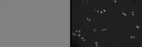

Segmentation

In order to track cells, we need to do segmentation first. In this method, we use seeded-watershed algorithm for cell segmentation.

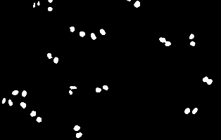
Binarization

In order to get a rough binary image with cell-classified pixel as foreground, we implement simple thresholding with empirical threshold value for coarse segmentation and morphological closing for hole filling.

img = cv2.GaussianBlur(img,(5,5),0).astype(np.uint8)
_, thresh = cv2.threshold(img, threshold, 1, cv2.THRESH_BINARY) # threshold = 50

kernel = cv2.getStructuringElement(cv2.MORPH_ELLIPSE,(9,9))
thresh = cv2.morphologyEx(thresh, cv2.MORPH_CLOSE, kernel)

The result of binarization:

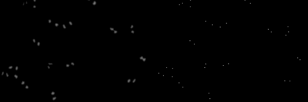
Distance Map

To do watershed, we need to find the seed point for each cell first, which is the center of cells. To detect these points, a simple way it to compute L2 distance map and maximum filter to extract the centers.

cv2.distanceTransform(image, distanceType=2, maskSize=0) # using L2 distance and use the percise mask
scipy.ndimage.filters.maximum_filter(image, neighborhood_size) # empirically set neighborhood_size to 20 (the min distance to the nearest cell)

The result is like this (left: distance map; right: seeds for watershed):

Watershed

Finally, it’s time to use watershed based on the seed points to segment cells!

_, labels = cv2.connectedComponents(seed_img) # use region growing label each seed
segmentation = cv2.watershed(combined_img, labels) # watershed

Note: the input image to watershed is not the normalized image, but the image combine with distance map with certain coefficient; in another word,

I_combined = I_normalized + a * I_distance

where a is set empirically as 0.4.

The result is like this (left: result of binarization; right: result of watershed):

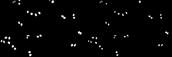
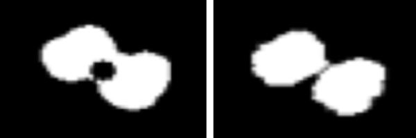
Watershed can segment the cells overlapping together (left: result of binarization; right: result of watershed):

Tracking

In this step, we implement the tracking algorithm based on the watershed results and normalized images.

Neighboring Graph Construction

The similarity of cell’s morphology makes it hard to track; therefore, understanding the spatial relationship with repect to each cell is significant to us, like the number of neighbours and the directions of those neighbours. In this method, we use Delaunay triangulation to build this kind of Neighboring Graph. OpenCV provides a cv2.Subdiv2D function for triangulation.

To implement triangulation, firstly, we need build the Subdiv2D instance:

# Rectangle to be used with Subdiv2D
h, w = image.shape[:2]
rect = (0, 0, h, w)
 
# Create an instance of Subdiv2D
subdiv = cv2.Subdiv2D(rect)

Afterwards, we need to find the center points for each cell and in our case, we compute the centroid for each cell region.

_, contours, _ = cv2.findContours(watershed, cv2.RETR_EXTERNAL, cv2.CHAIN_APPROX_TC89_KCOS) # find contours 
for contour in contours:
	m = cv2.moments(contour)
	if m['m00']:
	    centroids.append(( int(round(m['m01']/m['m00'])),\
	                       int(round(m['m10']/m['m00'])) ))

Lastly, we triangulate these points by:

for pt in centroids:
	subdiv.insert(pt)
	triangleList = subdiv.getTriangleList();
	for tri in triangleList:
		# pt1, pt2, pt3 are the three vertices of each triangular
		pt1 = (int(t[0]), int(t[1])) 
		pt2 = (int(t[2]), int(t[3]))
		pt3 = (int(t[4]), int(t[5]))

Result of triangulation:

Contour Analysis

To measure the distance of contours between cells, directly using its binary shape is a way, but in this method, we use Fourier Descriptors (FDs), instead, since reduce the sensitivity of using binary boundary by using the lower order of the descriptor. pyefd package provides the function for computing FDs.

We can get the parameters of FDs by:

_, contours, _ = cv2.findContours(watershed, cv2.RETR_EXTERNAL, cv2.CHAIN_APPROX_TC89_KCOS)
for contour in contours: 
	pyefd.elliptic_fourier_descriptors(contour, order=10, normalize=False) # we empirically choose the order as 10

Intensity Analysis

For intensity analysis, we use Co-occurrence Matrix (CM) to measure the texture of cells, since unlike simple histogram, CM not only provides the information of intensity amongst all pixels, but also includes the spatial feature, such as texture. In our case, we use 4-direction CM to build the texture feature. The implementation of this part is pretty straightforward and it’s little bit long; therefore, I’ll only describe some patches and for more details, please go to the Github repository and look into the ipynb code.

# convert the intensity from 0 - 255 to 0 - level (we set it as 10)
max_v, min_v = np.max(cell_patch_in_normalized_image), np.min(cell_patch_in_normalized_image)
range_p = max_v - min_v
img = np.round((cell_patch_in_normalized_image.astype(np.float32)-min_v)/range_p*level)

# initialize CMs
h, w = img.shape[:2]
p_0 = np.zeros((level,level))
p_45 = np.zeros((level,level))
p_90 = np.zeros((level,level))
p_135 = np.zeros((level,level))

... # scan each pixel in the patch of a single cell to build CMs
	
... # compute the Entropy, Energy, Contrast, Homogeneity for each CM	

Position

We describe the position of cells simply using centroids.

Mitosis Analysis

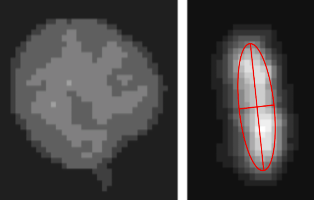
Since the cells in mitosis has unusually appearance in terms of intensity and boundary, we need to identify them when we compute the distance of disimilarity. To identify the cell in mitosis, the simple way it to identify the elongated cells, since that’s how they usually look like. To identify elongated shape, we use the ratio of major axis and minor axis of the eclipse of inertia for each cell.

_, contours, _ = cv2.findContours(cell_patch_in_binary, cv2.RETR_EXTERNAL, cv2.CHAIN_APPROX_TC89_KCOS)
(x,y),(minor,major),angle = cv2.fitEllipse(contours[0])
ratio = major / minor

The example of the cell in mitosis is shown below (left: the cell in previous frame; right: the same cell in mitosis):

Matching

Finally, we have all of the features we need and then we can use these features to match (track) cells based of the disimilarity metrics: 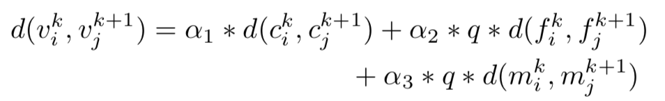where the meanings of each term in the right hand side are the distance of centroid, the difference of FDs and the difference of CMs. For more details, please look into the technical report in the Github repository.

The final result:

The example of tracking the cell in mitosis.

The plot of the previous tracking.

Done!